Engineering Mathematics I

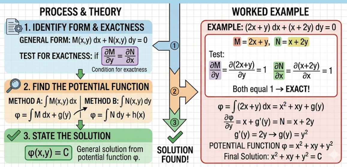
First Order Exact Equations

• General form:M(x,y) dx + N(x,y) dy = 0.
• Exact if∂M/∂y = ∂N/∂x.
• Solution obtained from the potential functionφ(x,y) = C.
• Example:(2x + y) dx + (x + 2y) dy = 0is exact since both mixed derivatives are 1.

Diagram: exact-ode-flow.png

First Order Linear Equations

• Standard form:dy/dx + P(x) y = Q(x).
• Integrating factor:IF = e^(∫P(x) dx).
• Solution:y IF = ∫Q(x) IF dx + C.
• Example:dy/dx + y = e^x → IF = e^x.

Bernoulli Equations

• Form:dy/dx + P(x) y = Q(x) y^n.
• Converted to linear usingv = y^(1-n).
• Example:dy/dx + y = y^2 → v = y⁻¹.

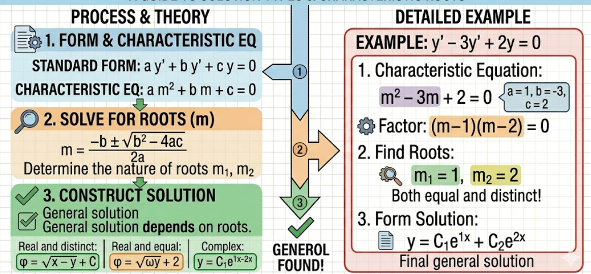
Second Order Linear Equations with Constant Coefficients

• Standard form:a y'' + b y' + c y = 0.
• Characteristic equation:a m^2 + b m + c = 0.
• Solution based on roots:
• Real and distinct:y = C1 e^(m1 x) + C2 e^(m2 x).
• Real and equal:y = (C1 + C2 x) e^(mx).
• Complex:y = e^(αx)(C1 cos βx + C2 sin βx).
• Example:y'' - 3y' + 2y = 0 → roots 1 and 2.

Diagram: characteristic-roots.png

Method of Variation of Parameters

• Used for non homogeneous equationsy'' + P y' + Q y = R.
• Requires complementary function (CF) from the homogeneous part.
• Particular integral (PI) obtained by varying constants in CF.
• Example:y'' + y = sin x.

Euler (Cauchy) Equations

• Form:x^2 y'' + a x y' + b y = 0.
• Substitutionx = e^tconverts it to constant coefficient form.
• Example:x^2 y'' - 3x y' + 3y = 0.

Systems of Differential Equations

• Linear systems can be solved by elimination or matrix methods.
• Example:dx/dt = x + y , dy/dt = x - y.